Gerrymandering
The MGGG held their 2nd satellite workshop on the Geometry of Redistricting at Duke, 2-5 November 2017. Beyond the fancy name, this was a workshop to learn about gerrymandering (how it is done, how to spot it) and to look at how mathematics can help understand what we see (simple metrics, up to advanced tools). The first two days were devoted to the public workshop and the last two days were devoted to 3 specialty tracks: expert witness training, educator training, and a hackathon. I participated in the Hackathon (my first) and enjoyed the experience thoroughly.
Hackathon
Although the overall Workshop series was lead by Moon Duchin and hosted at Duke by Jonathan Mattingly, the Hackathon was led by Sarah Huggenberger and Blake Esselstyn. We had been given a list of projects in advance and I was looking to work on one that had a connection to the people who were dealing with gerrymandering. The one project that jumped out was called “Preliminary Analyses on Local Election Data”, involving a (new to me) technique called “Ecological Inference”, but importantly it had been requested by a several civil rights groups as a way to look for vote dilution.
Not to get into the weeds too much, but the in the case of Thornburg v. Gingles, the US Supreme Court established the Gingles test, in which 3 conditions needed to be satisfied in order to establish vote dilution:
- Geographical compactness of minority group
- Politically cohesive minority group
- Majority votes as a block in opposition to the minority group
The idea behind this project was to develop a tool that gave the interested parties more insight into whether these conditions had been met, using census and voting data.
Since we were on the 2nd satellite workshop, a good start had been made by the Hackathon at the 1st workshop and so we had a Shiny app (written in R) as a starting point. It took a file of census and voting information and calculated the white vs black support using three modes of attack:
- The homogeneous precincts assumption
- Goodman’s Ecological Regression
- Ecological Inference
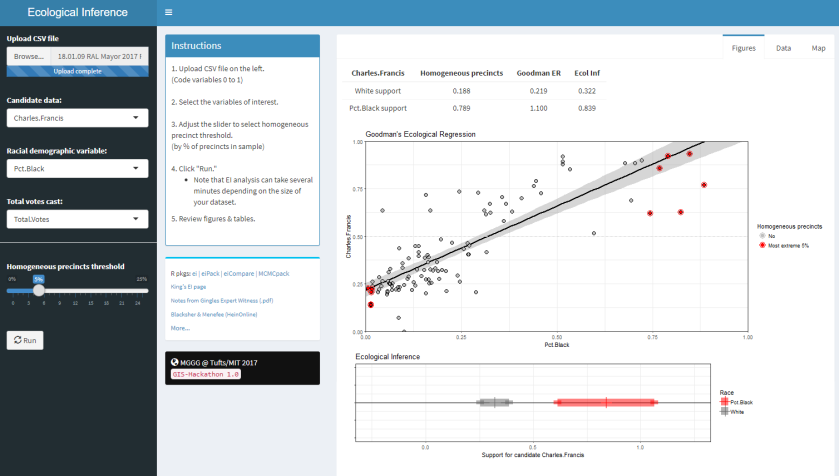
My aspect of this Hackathon was to extend this Shiny app was to add GIS shapefiles and then to map the data for each precinct onto them.
Side-note: Inferring Individual Behavior from Aggregate Data
We want a technique to infer something about a population based on knowledge of only macro information of the size of the population and distribution of the population in the subgroups within a region.
Formally the problem can be written as the number of people in group P doing task Q:
T = β*X + γ*(1-X)
where
- T = the proportion of people doing task Q (known)
- 1-T = the proportion of the people not doing task Q
- X = the proportion of the people in group P (known)
- 1-X = the proportion of the people not in group P
- β = the proportion of people in group P doing task Q (unknown)
- γ = the proportion of people not in group P doing task Q (unknown)
The simplest solution is to assume that a subset of regions that have above a threshold of a certain demographic proportion (X > 90% or 1-X > 90%, for example) are essentially homogeneous (giving rise to the name Homogeneous Precincts [1]), and to make statements for all regions based on the aggregates of these regions (β = T or γ = T, respectively). The problem with this analysis technique is that there are usually proportionally few regions that satisfy the criteria for the threshold, and the relative sizes of the populations many not be representative of other factors.
Another slightly more complicated solution is to establish upper and lower bounds for β & γ based on the extremes of the proportions on the people in the two groups, known as the Method of Bounds [2].
- Assume that none of the people not in group P did task Q (all of the people doing task Q came from group P): set γ = 0 and solve for β = T/X
- Assume that all of the people in group P did not do task Q: set γ=1 and solve for β=(T+X-1)/(X)
Thus we get β = [T/X, (T+X-1)/X] for γ=[0, 1]. While accurate mathematically, it is difficult to answer a question with precision when bounds are involved for every region.
A slightly more robust process is Ecological Regression [2], in which the equation above is multiplied out to give:
T = γ + (β-γ)*X
which is similar to the equation for a straight line in X & T:
T = b + m*X + ε
where ε = a general error term. If data for all regions in question are used as input data for a linear regression, a representative line can be drawn for all regions simultaneously. The hiccup in this process is that “b” can be larger 1.0 or smaller than 0, which can be difficult to explain away to a non-mathematician — “how can you have more votes than people voting?”
A much more robust process is called Ecological Inference [3, 4], which assumes that
- there is one cluster of points (even if drawn out) on the unit square, following a truncated bivariate normal distribution
- there is an absence of spatial auto-correlation (the X’s and T’s are mean-independent)
- the X’s are independent of the β’s & γ’s
and then solves the original equations iteratively for each region to determine best values for β & γ. This technique has been implemented in R in the ei [5] and eiCompare [6] packages.
Additionally, although this side-note only gave the 2 x 2 factor case ([people in group P, people not in group P] x [people doing task Q, people not doing task Q]), the Ecological Inference model has been developed to include the R x C factor case [3].
Results
The process of adding the shapefiles was fairly straightforward, but several design ideas had to be honored:
- The original functionality would continue if a shapefile wasn’t specified
- The user would be allowed to specify which column in each file denoted the “precinct” for the maps. This was important because the shapefiles tended to have names that were important to the GIS technician who released the file, but could be difficult to change on the fly.
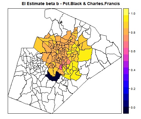
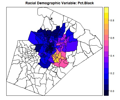
Below are screen shots of the original functionality being preserved and also of the added choropleths. This 2017 Raleigh mayoral election had an interesting twist in that there was one precinct in which no-one voted at all, leading it to be shaded dark blue in the ecological inference choropleths.
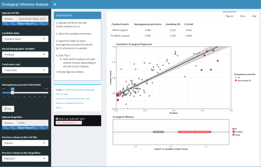
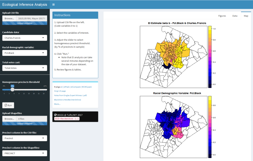
What was done:
- Added shapefile dialog to GUI
- Added a no-crash option of there is no shapefile
- Added common precinct column drop-downs to GUI
- This is required because we need to be able to join the data from the CSV file to the shapefile and we need to be told which columns have the precinct info in them
- Made the common precinct column drop-downs modal to having a shapefile selected
- Forked the data just after it is loaded (to prevent mashing of the original data)
- Calculated the EI estimate again with Betas TRUE
- Added plotting of the Betas on the upper map on the MAPS tab (Figure 4)
- Added plotting of the Racial Demographic on the lower map on the MAPS tab (Figure 5)
- Added tryCatch to the major operations
- Added comments and renamed some variables for readability
- Added 2017 Raleigh Mayoral election data as a data-set (real data!)
There are still some tasks that need to be completed
- Make the color ramps on the spplots nicer (the default ranges are based on the data, not on the [0, 1] interval)
- Change the code so that the first ei_est_gen can calculate the Betas (there are a lot of steps to this one)
- Fix the coercion warnings on the Joins for the Precincts (this will allow the tryCatch to be used)
- Build a dummy shapefile for and check the data vs cor_6 from the eiCompare package
- Add the calculated Betas to the DATA tab
Conclusion
Participating in the overall workshop and in the hackathon in particular was a lot of fun. I learned a lot about both gerrymandering also ecological inference. The shiny app advanced and although there are still some open items, a fair amount of progress was made. I’m looking forward to participating in the next Gerrymandr hackathon at Duke and continuing my involvement in the gerrymandering topic in the future.
End-notes:
- Ards, S & Lewis, M (1992) “Vote Dilution Research: Methods of Analysis,” Trotter Review: Vol. 6: Iss. 2, Article 9.
- Kousser, J. M., (2001) “Ecological Inference from Goodman to King”, Historical Methods: Summer 2001: Vol 34: No. 3, pgs 101-126
- King, G., (1997), “A Solution to the Ecological Inference Problem”, Princeton University Press
- King, G., Rosen, O., Tanner, M., (2004) “Ecological inference : new methodological strategies”, Cambridge University Press, pgs 6-7
- King, G. & Roberts, M., (2016), “Package: ei”, CRAN Repository
- Collingwood, L., (2017), “Package: eiCompare”, CRAN Repository